Machine Learning Algorithms for Business Applications – Complete Guide

With the development of free, open-source machine learning and artificial intelligence tools like Google’s TensorFlow and sci-kit learn, as well as “ML-as-a-service” products like Google’s Cloud Prediction API and Microsoft’s Azure Machine Learning platform, it’s never been easier for companies of all sizes to harness the power of data. But machine learning is such a vast, complex field. Where do you start learning how to use it in your business?

In this article, we’ll survey the current landscape of machine learning algorithms and explain how they work, provide example applications, share how other companies use them, and provide further resources on learning about them. This executive overview will provide the first step in learning how to apply machine learning algorithm(s) to make your business more efficient, more effective, and more profitable.

As you read through the examples below, you might want to jot down business challenges that are analogous to the problems that these algorithms can solve—perhaps an algorithm that predicts the occurrence of safety issues in coal mines can also be used to predict which of your restaurant franchises are at risk for non-compliance with health regulations. By the end of this article, you’ll have an action plan of which algorithms to research further and a solid grasp of their potential to provide concrete benefits to your bottom line.

Classification

Goal: The goal of classification algorithms is to place items into specific categories and answer questions like: Is this tumor cancerous? Is this email spam? Will this loan applicant default? What category of article is this? Which demographic does this online customer fall into?

Bayesian Classifier

Bayesian Classifiers are a simple yet highly effective classification algorithm. They are based on Bayes’ Theorem, which succinctly defines the probability of an event given that another related event has occurred. A Bayesian Classifier categorizes data by keeping track of the probabilities that specific features—characteristics of a data set that you believe may impact its classification—accompany a specific classification.

While Bayesian Classifiers can be used for any classification task, they are particularly useful with document classification, especially spam filters. For instance, Computer Scientist and famed Startup Investor Paul Graham developed a simple Bayesian spam filter that caught over 99.5 percent of his spam while having no false positives (non-spam emails mistakenly marked as spam). The features Graham used included the words in the emails, the email headers, and the presence of embedded HTML and JavaScript.

Graham provides a nice illustration of how the spam filter works by extracting the 15 most interesting features, or the 15 features that were either the most powerful indicators of spam (a weight close to 1.0) or the weakest indicators of spam (a weight close to 0.0).

The following chart organizes the interesting features in one of Graham’s spam emails:

Feature	Value	Interpretation
madam	0.99	Spammy
promotion	0.99	Spammy
republic	0.99	Spammy
shortest	0.05	Not-Spammy
mandatory	0.05	Not-Spammy
standardization	0.07	Not-Spammy
sorry	0.08	Not-Spammy
supported	0.09	Not-Spammy
people’s	0.09	Not-Spammy
enter	0.91	Spammy
quality	0.89	Spammy
organization	0.12	Not-Spammy
investment	0.86	Spammy
very	0.15	Not-Spammy
valuable	0.82	Spammy

Combining these probabilities via Bayes’ Rule results in a probability of 0.90, meaning the email is most likely spam.

Bayesian Classifiers are effective even with complex document classification tasks. A Stanford study showed a Naïve Bayes Classifier (the “naïve” comes from the classifier assuming every word’s appearance is independent of every other word’s appearance) was 85% accurate in sentiment analysis of Tweets. Another study at MIT found a Naïve Bayes Classifier could accurately categorize articles in the MIT student newspaper 77% of the time. Other potential applications include authorship identification and even predicting whether a brain tumor could relapse or progress after treatment.

Pros:

• Often perform as well as much more complex algorithms but while being easy to implement. This makes Bayesian Classifiers a good first-line machine learning algorithm.
• Simple to interpret. Each feature has a probability, so you can see which are most strongly associated with certain classifications.
• An online technique, meaning it supports incremental training. After a Bayesian Classifier is trained, each feature has a specific conditional probability attached to it. To include one new data sample, you simply update the probabilities–no need to go through the original data set all over again.
• Very fast. Since Bayesian classifiers are simply combining pre-calculated probabilities, new classifications can be made very quickly even on large and complex data sets.

Cons:

• Can’t deal with outcomes dependent on a combination of features. The assumption is that each is independent of each other—which can sometimes lower accuracy. For example, the words “online” and “pharmacy” may not normally be a strong indicator of spam in an email unless the words are used together. A Bayesian Classifier would not be able to pick up on that interdependence of those two features.

Decision Tree Classifier

Decision Trees are perhaps the most intuitively understandable machine learning algorithm, because in essence they are flowcharts in software form. Decision Trees classify items using a series of if-then statements that eventually result in a classification.

A simple example: You come across a beverage at a restaurant, and want to figure out what type of beverage it is. A Decision Tree could classify the beverage based on the results of the following questions:

Is the beverage hot or cold?

It’s cold.

Is it caffeinated or caffeine free?

It’s caffeinated.

Is it carbonated (“fizzy”)?

It’s not carbonated.

Was it made with beans or leaves?

It was made with leaves.

Final classification: iced tea

The key to an effective decision tree is to have statements that divide the dataset well—that is, the more homogenous the data is after each division, the better that division is. There are multiple metrics that can be used to determine how to split a decision tree—two common ones are entropy and Gini impurity. Using an algorithm called CART (Classification and Regression Trees), each level of the tree is split via the attribute that causes the greatest reduction in the chosen metric. This process is repeated until further splits no longer reduce that metric, and the tree is complete!

A more substantive application of a decision tree could be predicting user signups. Suppose you run a subscription service, and your system logs several characteristics about your users who’ve signed up for the free trial – whether they’ve tried your interactive demo, whether they’ve signed up for your mailing list, how they found your website (search engine, social media, etc.), and whether they ultimately signed up for the paid version of your service.

A decision tree could not only use this data to predict which new free trial users would ultimately become paying customers, but also show you the exact funnel which led them there; perhaps it was social media -> mailing list -> paid subscription, which indicates your demo is hurting your conversion rate while your social media presence is bringing in paying customers.

Other example applications: BP used a decision tree to separate oil and gas and “replace a hand-designed rules system…[the decision tree] outperformed human experts and saved BP millions.” A MIT study examined how decision trees could be used to predict whether an applicant would receive a loan, and whether that applicant would default.

Pros:

• Very easy to interpret and explain. Decision Trees mirror human decision-making through their flowchart “if-then” style of splitting data down until the data is categorized.
• Can be displayed graphically. A decision tree is, in essence, a branching flowchart (just one that’s been algorithmically tuned for optimal splits), and smaller decision trees displayed graphically can be easily interpreted even by non-technical people.
• Can easily use both categorical and numerical data; e.g, is this car red works just as well as, “Is the car’s tire diameter between six and eight inches”? In other classifiers, you’d have to create a “dummy” variable to work around this.
• Can deal with interactions of variables. In the “online pharmacy” example that stumped the Bayesian Classifier above, a decision tree could split the data set on whether it contained the world “online”, and the split the result by whether it contained “pharmacy”, ensuring that “online pharmacy” = spam while “online” and “pharmacy” = non-spam.

Cons:

• Decision Trees may not be as accurate as other classification algorithms as they have tendency to “overfit” the data (meaning they make excellent predictions within the data set used to train them, but poorer predictions for new data coming in). Nonetheless, there are various methods of “pruning” the tree to improve accuracy.
• Decision Trees are not an online technique, meaning the whole tree must be recreated from scratch in order to incorporate new data, since the variables that optimally split the data could change.
• With larger data sets the number of nodes on a decision tree can grow extremely large and complex, resulting in slow classifications.

Support Vector Machines

Support Vector Machines (SVMs) are a complex but powerful classification technique. Working on numerical data, SVMs classify by finding the dividing line (formally called a maximum-margin hyperplane) that separates data most cleanly. This is not always inherently obvious, so sometimes polynomial transformation (transforming the data onto different axes–for example, instead of plotting GPA vs. SAT score for predicting if a student is admitted to a certain university, you may transform the data by plotting GPA-squared vs. SAT score squared) is used to transform data to a different space, where the dividing line will be more clear.  

Classification is based on which side of the dividing line new data falls. This can get very complex even for technical people, though once the SVM is constructed it’s fairly simple to use. While most commonly used for classification problems, SVMs have been extended to regression tasks in more recent years.

Example: SVMs are often used with very complex data for applications such as recognizing handwriting, facial expression classification, and classifying images. For example, an SVM could recognize numerals written in the Arabic/Persian script with a 94% accuracy. In this case, there were 10 classes (0, 1, 2, 3…9), and the SVM operated on a digit-by-digit case to classify each handwritten digit into one of those classes. In this case, the SVM was more accurate the a Neural Network.

The complexity of choosing the features–in this case, another algorithm was used for “feature extraction” which involved the proportion of white pixels in each image of a handwritten digit–makes this sort of problem more suitable for a SVM than, say, a Bayesian Classifier, where features are typically well identified beforehand.

Pros:

• Very fast at classifying new data. There is no need to go through training data for new classifications.
• Can work for a mixture of categorical and numerical data
• SVMs are “Robust to high dimensionality”, meaning they can work well even with a large number of features.
• Highly accurate.

Cons:

• Black box technique. Unlike Bayesian Classifiers and Decision Trees, SVMs don’t offer easily digestible data “under the hood”. A SVM can be a highly effective classifier, but you may not be able to figure out why it makes those classifications.
• Typically requires a very large dataset. Other methods, like decision trees, can still give interesting output for small data sets; this may not be the case with a SVM.
• SVMs are not online. They will need to be updated every time new training data is to be incorporated.

Neural Networks

Neural Networks make both numeric (see next section) and classification predictions by loosely imitating the way the brain processes information.

In the human brain, neurons transmit information by forming connections with other neurons and transmitting electrochemical signals through these neural networks. Artificial Neural Networks, (also more simply called Neural Networks or Neural Nets)

There are many different kinds of Neural Networks, so to keep things simple we’ll look at just one called a Multilayer Perceptron Neural Network (MLP NN). A MLP NN contains at least three (but often more) layers of neurons: the input layer, one or more hidden layers, and an output layer. The input layer consists of the data you’re using to generate the prediction. The hidden layers, named because they don’t directly interact with either input or the final output, work on the data fed to them by the previous layers, and the output layer is the final prediction produced by the algorithm.

These layers are connected by synapses (named after the corresponding structure in real-life brains that allow electrochemical signals to pass between neurons). These synapses have weights, which, in combination with the inputs, determine which neurons in the subsequent layer are activated, which in turn affect which neurons in the next layer are activated, and so on.

The final layer of neurons feeds their results to the outputs, and whichever output is strongest (the classification most strongly associated with the input, for example) is the algorithm’s prediction. The operation of the hidden layers can be particularly mysterious to the untrained eye and, as explained below, even experts can’t develop meaningful interpretations of their output.

Synapse weights can initially be assigned randomly, and are then trained through a technique known as back propagation. The MLP NN is fed data for which the correct result is known–for instance, an image of a tiger and the classification “tiger”. If the MLP NN misclassified the image, the weight of the synapses that would have lead to a “tiger” classification are slightly increased, while the weight of the synapses that lead to other classifications are slightly decreased. With enough training data, the synapse weights eventually converge to their optimal values, and (ideally) the MLP NN now classifies tiger images with a high level of accuracy.

While unarguably the most complex machine learning algorithm discussed here, Neural Networks are also the most exciting and active area of machine learning research today. With the massive increases in datasets and computational power now available today, Deep Learning, which features Neural Networks with many layers, can be applied to many complex datasets like audio and images.

There is no dearth of applications for Neural Networks, and some of the biggest players in the industry are applying them toward cutting-edge solutions: Amazon uses Neural Networks to generate product recommendations; Massachusetts General Hospital uses deep learning to improve patient diagnosis and treatment; Facebook uses deep Neural Networks for facial recognition; Google powers Google Translate with Neural Networks.

Pros:

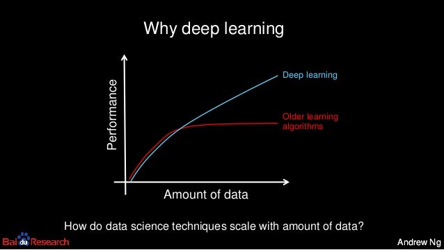
• Highly scalable. With massive datasets, other algorithms can (eventually) plateau in performance (see this image from this slideshow presented by Dr. Andrew Ng, Chief Scientist at Baidu), while Neural Network performance can keep improving.
• An online method. Neural Networks can be incrementally trained with new data.
• Space efficient. Like Bayesian Classifiers, they are represented by a list of numbers (for Bayesian Classifiers, this list represents feature probabilities; for Neural Networks, they represent synapse weights)

Cons:

• Black box method. In large Neural Networks with many thousands of nodes and an order of magnitude more of synapses, it’s difficult if not impossible to understand how the algorithm determined its output.
• The sheer level of complexity of Neural Networks, as demonstrated even in this highly simplified explanation of them, means that highly-skilled AI researchers and practitioners are needed to properly implement them.

Logistic Regression

Logistic regression is a classification algorithm that uses the properties of the logistic function (sometimes also called the sigmoid function), a “S” shaped curve that is typified by plateaus on both edges of the function and rapid growth in the middle. Weights are assigned to features and then fed to the logistic function, which outputs a number between 0 and 1. The decision boundary determines the classification. For example, if you’re using logistic regression to predict fraudulent credit card transactions, you may determine that an output below 0.5 is a legitimate transaction, while an output above 0.5 is a fraudulent transaction. Your decision boundary is 0.5.

The key to logistic regression is training the model to assign appropriate weights to all the features. This first requires a cost function, which is simply a function that determines the level of error of each prediction compared to the training example.

The most common cost function in logistic regression is sum of squares error (also called residual sum of squares). Then, using a calculus technique known as gradient descent, the weights are continually adjusted until the cost function is minimized. At this point, the logistic regression classifier is optimally accurate for predicting results in the training set, and this is the starting point for using it to predict classifications for new data.

Logistic regression can be extended to data with more than two categories (called multinomial logistic regression), by using a “one-versus-all” model. To classify, say, three types of documents–receipts, memos, customer mail–multinomial logistic regression would run three times, first classifying documents as “receipts or not-receipts”, then “memos or not-memos”, and finally “customer mail or not-customer mail”, and combine these results to make predictions.

Like Bayesian Classifiers, logistic regression is a good first-line machine learning algorithm because of its relative simplicity and ease of implementation. A few example applications include analysis of sheet metals, predicting safety issues in coal mines, and various medical applications.

Pros:

• Easy to interpret. Logistic regression outputs a number between 0 and 1, which can loosely be interpreted as a probability (0.312 could be interpreted as 31.2% chance of a credit card transaction being fraudulent). The feature weights easily indicate which features are more important in determining the classifications than others.

Cons:

• Is prone to overfitting. Logistic regression may require a fairly large training set before it can make accurate predictions outside of the training set.
• Not an online technique. Incorporating new data requires running gradient descent again.
• Has tradeoffs with gradient descent. The faster gradient descent determines the final feature weights, the more likely it is to miss the optimal weights. It can sometimes be difficult to figure this out the optimal speed versus accuracy tradeoff, and trial-and-error can be time consuming
• Dummy variables required for categorical data. Because logistic regression only produces real-valued output, categorical data must be converted to real values via a dummy variable (for instance, converting “red or not red” to “1 or 0” where red = 1, not red = 0).

Linear Regression

Linear regression is a familiar algorithm that attempts to create a line of best fit for a dataset and use that line to make new predictions. It’s the linear function (think y = mx + b from high school algebra, where x is the feature and m is the feature weight) that minimizes the error as determined by the cost function (typically the sum squared errors function). Simple linear regression only uses one variable and is thus limited in its scope, but multivariable linear regression can handle much more complex problems. Like logistic regression, gradient descent is often used to determine optimal feature weights.

There are many possible applications for linear regression, such as predicting real estate prices, estimating salaries, predicting financial portfolio performance, and predicting traffic. In some cases, linear regression is used in combination with other, more sophisticated techniques to produce more accurate outcomes that those provided by any individual algorithm alone.

Pros:

• Easy to implement and interpret. Linear regression is much like logistic regression in terms of implementation difficulty, but linear equations are much more intuitive to humans than the logistic function.

Cons:

• Gradient descent tradeoff. Like Logistic regression, gradient descent requires a tradeoff between speed and accuracy, and getting it right may take many iterations of trial-and-error.
• Not an online technique. Incorporating new data requires running gradient descent again.
• Dummy variables required for categorical data. Because linear regression only produces real-valued output, categorical data must be converted to real values via a dummy variable (for instance, converting “red or not red” to “1 or 0” where red = 1, not red = 0).

K-nearest Neighbors

Suppose you had a fairly rare baseball card that you wanted to sell on eBay. How would you determine a good selling price? You may check what that card (or similar cards) is has recently sold for, and price your card in that range.

That’s essentially how K-nearest neighbors works. It compares a new piece of data to data with similar values, and then averages “nearby” items to predict the new data’s value. “Distance” between data points is determined by metrics such as Euclidean Distance or Pearson Correlation.

The “K” in K-nearest neighbors is a placeholder value for the number of nearest values averaged to make the prediction. The algorithm can also use weighted averages, where values nearby are weighted more heavily in determining the average. Variables may need to be scaled–for example, when predicting house prices using number of bedrooms and square footage, you may choose to use square footage and number of bedrooms multiplied by 1000 in order to keep the two variables on the same scale.

K-nearest neighbors can be used for predicting home prices (as demonstrated in the simplified example above), the prices of goods in marketplaces (as with the baseball card example above), and be used to make product recommendations.

Pros:

• Online technique. Like a Naïve Bayes classifier, K-nearest Neighbors supports incremental training
•  Can handle complex numerical functions while still being easy to interpret. You can see exactly which neighbors are used for the final predictions.
• Useful if data is difficult/expensive to collect. The scaling process can reveal which variables are unimportant for making predictions and thus can be thrown out.

Cons:

• Requires all training data to make predictions. This means K-nearest Neighbors can be very slow for large datasets and can require a lot of space
•   Finding correct scaling factors can be tedious and computationally expensive when there are millions of variables.  

Wrap Up

Now that you’re more familiar with common machine learning algorithms and their applications, what are the next steps in using this knowledge to help meet your business objectives?

First, identify your business needs and map them to the corresponding machine learning tasks. Want to get real-time data on whether social media posts about your company are positive or negative? That’s a classification task. Want to predict what your real estate holdings will be worth next year? That’s a regression task.

Second, review the above algorithms and research more deeply into the ones that are relevant. While specialists—such as machine learning engineers, data scientists, and AI researchers—may be needed to optimize and perfect these algorithms for your specific use case, many off-the-shelf tools and products are available for you to get started, such as:

1. TensorFlow, Google’s open-source AI framework
2. scikit-learn, an open-source Python machine learning library
3. Google’s Cloud Prediction API, part of Google’s Cloud Platform
4. Azure Machine Learning, part of Microsoft’s cloud offerings
5. Cloudera, a big-data platform with in-built management and data capabilities

It’s important to note that, due to space/scope limitations, there are a few machine learning algorithms and topics we didn’t cover here:

• Optimization algorithms, such as genetic algorithms and simulated annealing, which help find optimal solutions to problems with constraints. Example application: Maximizing airline revenue.
• Clustering algorithms, like K-means clustering, which discover groupings of data. Example application: Identifying clusters of women on a dating site to maximize matches.
• Recommender Systems, which is the application of a hodgepodge of algorithms, including some mentioned above, to make product recommendations or find users/products that are similar to each other. Example application: Recommending products to users on Amazon.com.

Interested in learning more about how you can apply machine learning to your business or industry? The following Emerj guides and articles are a good place to start:

1. Artificial Intelligence and Security: Current Applications and Tomorrow’s Potentials
2. How to Apply Machine Learning to Business Problems
3. Machine Learning and Finance – Present and Future Applications
4. Machine Learning Healthcare Applications — 2016 and Beyond
5. Machine Learning Industry Predictions: Expert Consensus
6. Machine Learning in Robotics – 5 Modern Applications
7. Predictive Analytics and Marketing — What’s Possible and How it Works
8. The State of Machine Learning and Predictive Analytics for Small Business

 

Image credit: Strategic Learning Transformation